")
")
Preliminary Remarks
The following detailed derivation largely follows the publication by Peter Filß.
A 200 l drum is assumed as the container. However, the derivation can be applied to any other cylindrical objects for which the corresponding assumptions hold.
The fundamental idea of the derivation is based on the field of view of the detector inside the container. This is defined by the collimator used and corresponds to the area of the active matrix from which radiation can, in principle, enter the detector. The volume within the detector's field of view is divided into small volume elements ΔV that are perpendicular to the collimator axis. For each of these non-overlapping volume elements that occupy the entire area of the field of view in the container, its contribution to the count rate in the detector is determined and all contributions are summed. A significant point is the transition from a finite thickness of the volume element to an infinitesimally thin volume element.
Note:
In the derivation, a cylindrical collimator is assumed. For other collimator geometries (e.g., conical, rectangular, etc.), corresponding adjustments need to be made in the derivation.
For the derivation, the detector is initially assumed to be point-like. The efficiency calibration is carried out using a calibration source that is also assumed to be point-like, located on the collimator axis at a distance S0 from the detector. Let the activity of the point source be A0. Then, the energy-dependent calibration factor K(E) can be determined from the measured count rate Z0 for a characteristic line at energy E with the emission probability η.
\[ Z_0=\frac{K}{4 \cdot \pi \cdot S_0^2} \cdot \eta_0 \cdot A_0 \]
\[ K=\frac{4 \cdot \pi \cdot S_0^2}{\eta_0} \cdot \frac {Z_0}{A_0} \]
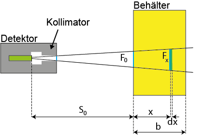
The starting point of the derivation is the area F0. This is defined by the area that the field of view of the collimator occupies on the side of the waste container facing the detector. For a corresponding cross-sectional area Fx in the waste container at a distance x from the outer side of the container, the inverse square law holds:
\[ \frac{F_0}{F_x} = \frac {S_0^2}{\left(S_0 + x \right)^2} \]
If CA is the activity concentration in the active matrix, η is the emission probability of the considered line, and µ is its linear attenuation coefficient, then the contribution to the count rate dZ of a cross-sectional area Fx of thickness dx can be expressed as
\[ dV = F_x \cdot dx \]
considering the attenuation of the emitted radiation over the distance x towards the detector as
\[ dZ = K \cdot \frac{\exp \left( -\mu \cdot x \right)}{4 \cdot \pi \cdot \left( S_0 + x \right)^2 } \cdot C_A \cdot \eta \cdot dV \]
This determines the contribution to the count rate dZ:
\[ dZ = K \cdot \frac{\exp \left( -\mu \cdot x \right)}{4 \cdot \pi \cdot \left( S_0 + x \right)^2 } \cdot C_A \cdot \eta \cdot F_0 \cdot \frac{\left(S_0 + x \right)^2}{S_0^2} \cdot dx \]
\[ dZ = K \cdot \frac{\exp \left( -\mu \cdot x \right)}{4 \cdot \pi \cdot S_0^2 } \cdot C_A \cdot \eta \cdot F_0 \cdot dx \]
\[ dZ = \frac{Z_0}{\eta_0 \cdot A_0} \cdot \exp \left( -\mu \cdot x \right) \cdot C_A \cdot \eta \cdot F_0 \cdot dx \]
To determine the count rate Z in the detector, the contributions of all areas Fx along x must be summed. In the transition
\[ \lim\limits_{x\to 0}dx \]
this corresponds to integrating the function dZ(x) for all \( x\in [0;h] \)
\[ Z=\int \limits_{0}^{h}dZ \]
After substitution and grouping the constant factors
\[ Z=\int \limits_{0}^{h}\frac{Z_0 \cdot F_0 \cdot C_A \cdot \eta }{\eta_0 \cdot A_0} \cdot \exp \left( -\mu \cdot x\right) \cdot dx \]
the integration yields
\[ Z=\frac{Z_0 \cdot F_0 \cdot C_A \cdot \eta }{\eta_0 \cdot A_0} \cdot \left[ -\frac{\exp \left( -\mu \cdot x\right)}{\mu} \right]_0^h \]
or
\[ Z=\frac{Z_0 \cdot F_0 \cdot C_A \cdot \eta }{\eta_0 \cdot A_0 \cdot \mu} \cdot \left[1 - \exp \left( -\mu \cdot x\right) \right] \]
The term in the square brackets is referred to as the correction factor K1 and describes the average attenuation along the total path length h.
\[ Z=\frac{Z_0 \cdot F_0 \cdot C_A \cdot \eta }{\eta_0 \cdot A_0 \cdot \mu} \cdot K_1 \]
The activity concentration CA can be expressed in terms of specific activity a and density ρ
\[ C_A = a \cdot \rho \]
Substituting into the preceding equation yields the expression for the count rate Z:
\[ Z=\frac{Z_0 \cdot F_0}{\eta_0 \cdot A_0 \cdot \mu} \cdot a \cdot \rho \cdot \eta \cdot K_1 \]
The constant terms can be summarized in the calibration factor H:
\[ H=\frac{\eta_0 \cdot A_0 }{Z_0 \cdot F_0} \cdot \left( \frac {\mu}{\rho} \right) \]
For specific activity a and activity A given the known mass M of the active matrix, the determination equations are derived
\[ a=\frac{H}{K_1} \cdot \frac{1}{\eta} \cdot Z \]
or
\[ A=M \cdot \frac{H}{K_1} \cdot \frac{1}{\eta} \cdot Z \]
Note:
The calibration factor H is connected to the mass attenuation coefficient \( \left( \frac{\mu}{\rho} \right) \) with the properties of the matrix. A simplification for practical handling occurs when an independent calibration quantity \( H^{'} \) is introduced.
\[ H=\frac{\eta_0 \cdot A_0 }{Z_0 \cdot F_0} \cdot \left( \frac {\mu}{\rho} \right) \]
This can be determined once for each measurement geometry, independent of the properties of the (later) quantifiable waste containers, for the relevant energy range. The respective matrix properties are considered multiplicatively through the mass attenuation coefficient.
\[ H = H^{'} \cdot \left(\frac{\mu}{\rho} \right) \]
In the two determination equations, envelopes of the active matrix are not considered. In general, the active matrix is contained in a container that may be surrounded by additional shielding layers, which is in turn encased by another container (e.g. waste drum).
The attenuation of the gamma radiation emitted by the active matrix in the N layers with thicknesses di is accounted for by an additional correction factor K2.
\[ K_2 = \exp \left( \sum \limits_{i=1}^{N} \mu_i \cdot d_i \right) \]
The determination equations multiplied by the correction factor K2 only describe the measurement of (specific) activity for a stationary measurement. In segmented gamma scan measurements, the collimated detector scans the waste container, meaning it is a dynamic measurement process. It is possible that the active matrix does not remain in the field of view of the collimated detector throughout the entire measurement. This characteristic is taken into account by the correction factor K3.
\[ K_3 = \frac{T}{T^{*}} \]
T is the total measurement time and T* is the time during which the collimated detector sees the active matrix.
Note:
This definition of the correction factor K3 applies only if the total measurement time T and the partial measurement time T* can be determined (e.g., from the information on segment spectra and spatial distributions). Often, alternatively, the ratio of the total scan height h to the height h* of the active matrix can also be used
\[ K_3 = \frac{h}{h^{*}} \]
The height h* can for example be inferred from analyzing the generated energy-specific spatial distributions.
Thus, the determination equations for measurements with collimated geometry for the specific activity a become:
\[ a = \left[ H^{'} \cdot \frac{1}{\eta} \cdot \left( \frac{\mu}{\rho}\right) \cdot \frac{K_2 \cdot K_3}{K_1} \right] \cdot Z \]
and the activity A with the mass M of the active matrix to
\[ A = M \cdot \left[ H^{'} \cdot \frac{1}{\eta} \cdot \left( \frac{\mu}{\rho}\right) \cdot \frac{K_2 \cdot K_3}{K_1} \right] \cdot Z \]
The expression in square brackets corresponds to the transfer function T.
